Timeseries Anomaly Detection
KDD Cup 2021 Multi-dataset Time Series Anomaly Detection competition (2nd place)
Challenge Overview
The competition focused on detecting anomalies across a highly diverse set of time series from various sources. Univariate time series anomaly detection is often highly dataset-dependent, making it challenging to identify algorithms that perform well across different datasets. The competition and accompanying dataset were designed to drive progress in academia and industry toward more generalizable solutions applicable to a wide range of anomaly detection scenarios.
Key details of the challenge include:
- 250 distinct time series datasets, each with highly varied characteristics.
- Each time series is split into training and test sets, with training data guaranteed to be anomaly-free and test data containing exactly one anomaly.
- All time series are univariate (single-dimensional).
- No anomaly labels were provided during the competition.
Proposed Solution
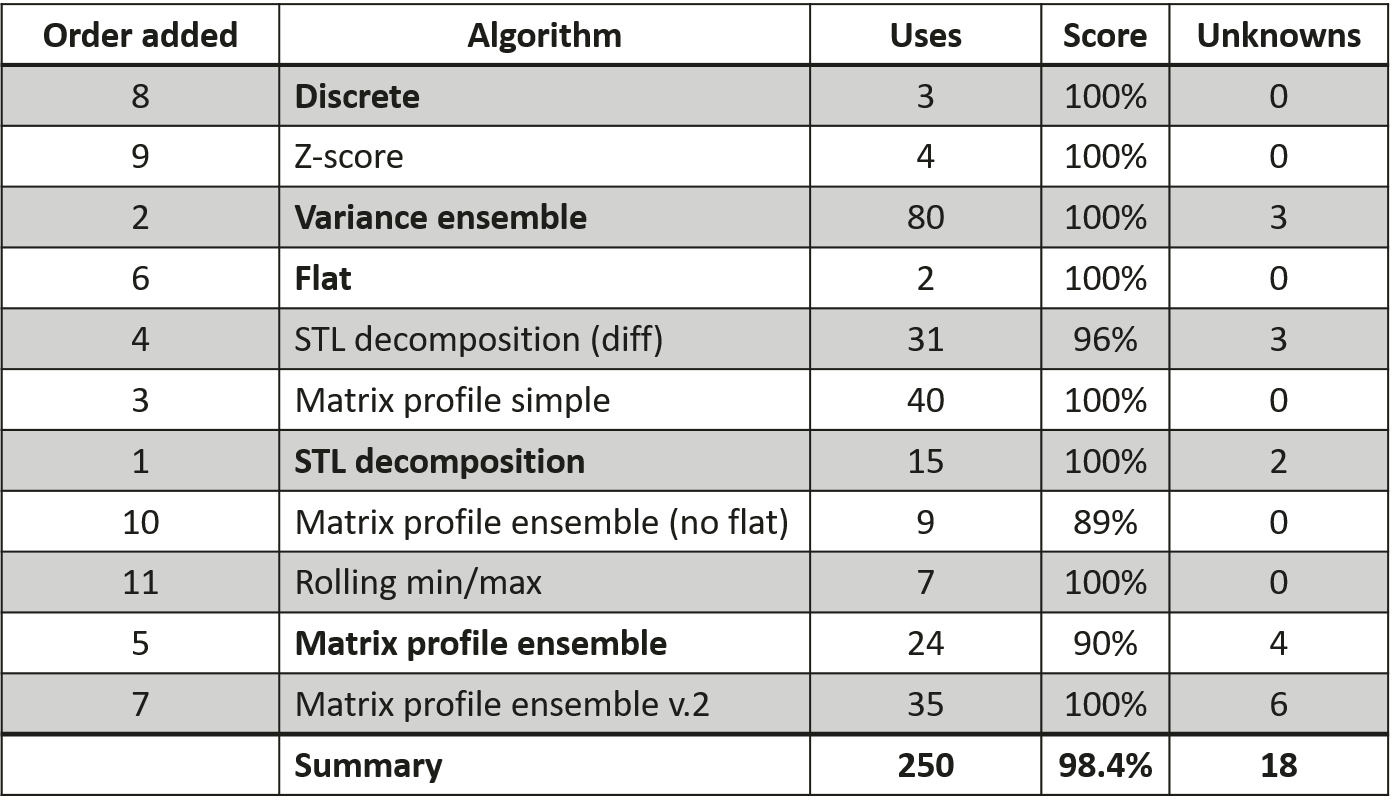
Our approach utilized a mixture-of-experts framework, applying a sequence of specialized algorithms, each tailored to detect specific types of anomalies (e.g., discrete, spike, discord, variance). These algorithms were applied in a fixed order, prioritizing those targeting simpler anomaly types and those with more conservative predictions, until a confident prediction was achieved. Our solution secured 2nd place out of 624 competing teams. A brief overview of our approach is available in a YouTube video.

The success of our multi-method solution relied on several key components:
- Confidence Measurement: A mechanism to assess the confidence of predictions for method selection.
- Period Inference: All time series in the dataset exhibit periodicity, though it may be irregular or multi-patterned. To simplify parameter selection, we base most model parameters on an inferred period. This approach ensures that time series with identical shapes but different sampling rates are treated consistently.
- Ensemble Learning: Recognizing that period inference may not always be perfect, we enhance robustness by testing a range of periods derived from the inferred period \(p\). Specifically, we consider a set of periods \(\{ f \cdot p \mid f \in \mathcal{F} \}\), where \(\mathcal{F}\) is a set of multipliers. For example, if a time series \(T\) has an inferred period \(p = 128\) and a method \(A\) uses multipliers \(\mathcal{F} = \{0.5, 1.0, 2.0\}\), we run method \(A\) with periods \(\{64, 128, 256\}\) and select the result with the highest confidence score.
Confidence Level

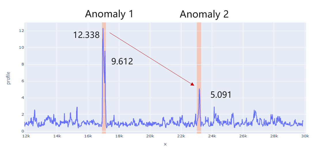
We calculate the confidence level by evaluating the difference between the maximum anomaly score and the second-highest score, excluding scores within the same peak (e.g., 9.612 in the figure is ignored). This difference is then compared to an algorithm-specific acceptance threshold. If the difference exceeds the threshold, the confidence level is greater than 1, and the prediction is accepted.
Using the example in the figure:
Difference: \(\frac{max(anomaly scores)}{(sec_max(anomaly scores)} − 1 = \frac{12.338−5.091}{5.091} = 1.423\)
Confidence (with a threshold of \(0.3\)): \(\frac{difference}{threshold} = \frac{1.423}{0.3} = 4.745\)
Since \(4.745 > 1\), the expert is deemed confident, and its anomaly prediction is accepted.
Experts
